Restoring focus to a blurred image

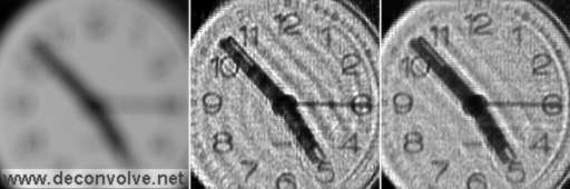
The figure above shows the results of using the BiaQIm image processing suite to 're-focus' an image of a clock that was taken with the camera lens out-of-focus. On the left is the original blurred image. The middle figure shows the results of applying non-blind saptially invariant PSF iterative deconvolution algorithm, using 64 iterations of the Biggs-accelerated Lucy-Richardson algorithm. The image has essentially been brought back into focus to the extent where you can now see not just the main numerals on the clock but also most of the fine minute divisions at the periphery. Note the ripples emanating from the dark clock handles. This is an example of a deconvolution artefact called ringing. Such ringing artefacts may partly be due to an imperfect PSF and the PSF used in this non-blind deconvolution was made by measurements on the camera that took the blurred picture (for more details about this and to see further examples, visit the 'Results' page of www.Bialith.com).
There are a number of ways to ameliorate ringing artefacts. One way is to refine the estimate of the PSF using myopic deconvolution. In the image on the right I have applied spatially variant myopic deconvolution to improve the estimate of the PSF at different locations in the image. This has reduced the ringing but not completely removed it. The lower the proportion of the solution energy is taken up by ringing artefacts, the greater the proportion that can be channelled into recovering the deconvolved solution. Hence effective measures to reduce ringing often produce more accurate deconvolution results. The fact that the ringing reduction is incomplete here may partly be due to me not using the 'best' parameters and constraints when setting up the spatially variant deconvolution. How to determine what is 'best' in this type of deconvolution is subject to ongoing research. Although this data is not provided in the demos downloadable from this site, you may download the blurred clock and PSF from www.Bialith.com if you want to try doing this experiment yourself.

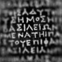
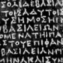
Above left is a portion of the rosetta stone blurred with a PSF kernel that gets larger as one goes further from the centre of the field. This simulates a kind of spherical aberration as seen with some lenses (e.g. microscope objective lenses). To correct this type of spatially variant blur you need to use spatially variant deconvolution and to the right you can see the results of applying an iterative spatially variant algorithm that is available in the BiaQIm image processing suite. More information on this example and other examples of spatially variant deconvolution can be seen at www.Bialith.com.

Blind deconvolution - restoring image and PSF simultaneously

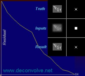
Above is a demonstration of the results seen using the Biggs-Andrews blind deconvolution method as implemented by the BiaQIm image processing suite. This method alternates between image restoration cycles and PSF restoration cycles and the BiaQIm image processing suite allows the blance of these cycles to be varied throughout the deconvolution procedure (at the time of writing - 25.5.2010 - I am unaware of any other software, whether commercial or free, that allows this). This data is available to download as one of the demo packages so you can try this out for yourself. The main figure is the residuals graph showing residual plotted against iteration (64 iterations in total are used here). Inset are the images. At the top are the ground truth data for image (left) and PSF (right). These ground truth images are not available to the algorithm but are shown here for comparason purposes. The actual input images to the blind deconvolution algorithm are shown in the middle - the blurred image (left) and our initial guess at the PSF (which is a simple flat square, right). The results of the blind deconvolution for image (left) and PSF (right) are shown at the bottom. The solution is good but note how the convergence is complex. Further examples of blind image deconvolution may be seen at www.Bialith.com.